
Overview
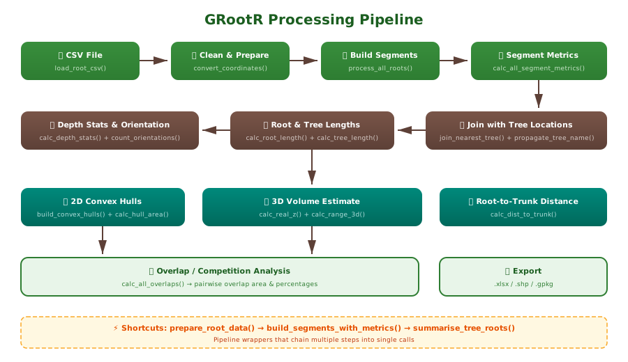
GRootR processes raw CSV data exported from GPR (Ground Penetrating Radar) software into spatial root segments, computes geometric and morphological metrics, and enables inter-tree root competition analysis.
Developed as part of the NCN-funded project: “Zastosowanie georadaru ze skanerem 3D do pomiarów zmienności systemów korzeniowych sosny zwyczajnej” (“Application of Ground-Penetrating Radar with 3D Scanner for Measuring Variability in Scots Pine Root Systems”)
Installation
# install.packages("pak")
pak::pak("j-miszczyszyn/GRootR")
Input data format
GRootR reads CSV files directly exported from GPR processing software (e.g., ImpulseRadar, REFLEXW, GPR-SLICE). A typical file looks like:
Spatial Reference System:,EPSG:2178,ETRS89 / Poland CS2000 zone 7,,,...
N.,Type,Name,Category,...,Node,X[SRS units],Y[SRS units],Depth[m],Altitude[m],Survey,...
1,Pipe,Feature 0010,Generic,...,node1,7394244.316,5578579.578,0.202,-0.202,Survey_2024.10.29_001_A_converted,...
,,,,,...,node2,7394245.057,5578579.786,0.202,-0.202,Survey_2024.10.29_001_A_converted,...
,,,,,...,node3,7394245.455,5578580.134,0.202,-0.202,Survey_2024.10.29_001_A_converted,...
2,Pipe,Feature 0011,Generic,...,node1,7394244.185,5578580.438,0.202,-0.202,Survey_2024.10.29_001_A_converted,...
Key points:
- Row 1 is CRS metadata (skipped automatically)
-
N.column is the root identifier — only filled in the first node of each root, empty for continuation rows (filled forward automatically) -
Nodecontains node labels likenode1,node2(ordering extracted automatically) -
X[SRS units],Y[SRS units],Depth[m]are coordinates -
Surveyis a composite string containing date, number, and plot ID
All column names are configurable — the defaults match this standard GPR export format.
Quick start
1. Load and prepare data
library(GRootR)

# One-liner — uses GPR export defaults
df <- prepare_root_data("path/to/gpr_export.csv")
Or step by step:
df <- load_root_csv("gpr_export.csv")          # skip=1, root_id_col="N."
df <- split_survey_column(df)                    # extracts plot ID from Survey
df <- convert_coordinates(df)                    # X[SRS units] → X, Y, Z
2. Build segments with metrics
segments <- build_segments_with_metrics(df, crs = 2178)3. Join with tree locations
library(sf)
trees <- st_read("trees.shp")

joined <- join_nearest_tree(segments, trees, tree_id_col = "Name", max_dist = 1.5)
joined <- propagate_tree_name(joined, tree_id_col = "Name")
4. Root and tree level metrics
joined <- calc_root_length(joined)
joined <- calc_tree_length(joined)
joined <- assign_depth_class(joined, bin_m = 0.2)
5. 2D/3D analysis
hulls    <- build_convex_hulls(joined, crs = 2178)
hulls    <- calc_hull_area(hulls)
z_range  <- calc_real_z(joined)
volume   <- calc_range_3d(z_range, hulls)
overlaps <- calc_all_overlaps(hulls)
All-in-one tree summary
summary <- summarise_tree_roots(joined, crs = 2178)
# Returns: $depth, $orientations, $hulls, $volume
Function reference
Loading & preparation
| Function | Description |
|---|---|
load_root_csv() |
Load GPR export CSV, skip header, fill N. → ROOT_ID
|
split_survey_column() |
Extract plot ID from composite Survey string |
convert_coordinates() |
X[SRS units] → X, Y[SRS units] → Y, Depth[m] → Z
|
prepare_root_data() |
All-in-one loader |
Segment creation
| Function | Description |
|---|---|
points_to_sf() |
Data frame → sf points (XYZ) |
make_segments() |
Consecutive points → line segments |
process_single_root() |
Process one ROOT_ID |
process_all_roots() |
Process all ROOT_IDs |
Segment metrics
| Function | Description |
|---|---|
calc_segment_length() |
3D Euclidean length |
calc_segment_azimuth() |
Bearing 0–360° |
calc_inclination() |
Angle from horizontal |
classify_slope() |
Slope category labels |
calc_all_segment_metrics() |
All of the above |
Tree joining
| Function | Description |
|---|---|
join_nearest_tree() |
Spatial join within distance |
propagate_tree_name() |
Propagate tree ID to all segments of same root |
Root / tree metrics
| Function | Description |
|---|---|
calc_root_length() |
Total length per ROOT_ID |
calc_tree_length() |
Total length per TREE_ID |
assign_depth_class() |
Depth bin classification |
calc_depth_stats() |
Max/mean depth, range per tree |
count_orientations() |
Vertical/horizontal segment counts |
Polygons & volume
| Function | Description |
|---|---|
build_convex_hulls() |
2D convex hull per tree |
calc_hull_area() |
Area + X/Y extent |
calc_real_z() |
Vertical range per tree |
calc_range_3d() |
3D bounding volume |
Overlap & distance
| Function | Description |
|---|---|
calc_all_overlaps() |
Pairwise root system overlap |
merge_root_segments() |
Union segments per root |
calc_dist_to_trunk() |
Distance root → tree stem |
Related publications
The methodology implemented in GRootR was developed during research on root system variability in Scots pine forests using multichannel ground-penetrating radar. The following publication presents the scientific background and first results obtained with the approach used in this package:
Tymińska-Czabańska, L., Polak, M., Miszczyszyn, J., Dąbrowski, M., & Socha, J. (2025). First application of multichannel GPR for root system variability analysis in Scots pine forests. Ecological Indicators, 179, 114282. doi:10.1016/j.ecolind.2025.114282
If you use GRootR in your work, please cite both the article and the package:
citation("GRootR")