
Overview
GRootR processes raw CSV data exported from GPR software through a pipeline that transforms point data into spatial segments with geometric metrics, 2D/3D morphology estimates, and inter-tree competition analysis.
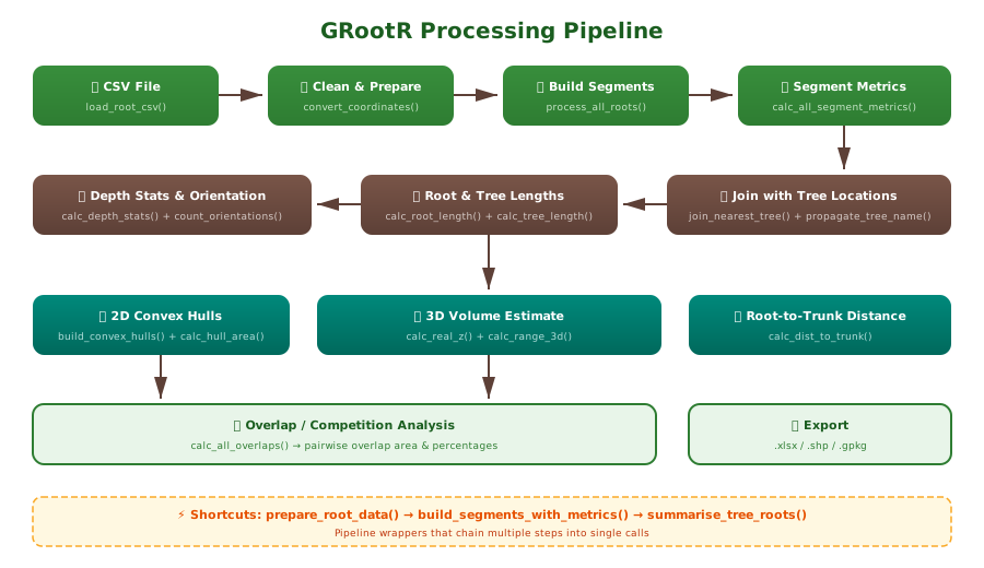
Installation
# install.packages("pak")
pak::pak("j-miszczyszyn/GRootR")
Step 1: Load and prepare data
The simplest approach uses prepare_root_data(). The
defaults match the standard GPR export format — just point to your
CSV:
library(GRootR)

df <- prepare_root_data("path/to/gpr_export.csv")
Or step by step:
df <- load_root_csv("gpr_export.csv")   # skips CRS header, fills N. -> ROOT_ID
df <- split_survey_column(df)            # extracts plot ID from Survey column
df <- convert_coordinates(df)            # X[SRS units] -> X, Y, Z
What happens internally:
-
load_root_csv()— skips the CRS metadata header row, reads the CSV, and fills missingN.values (the root identifier only appears in the first row of each root — continuation rows are empty) -
split_survey_column()— extracts the plot identifier from the composite Survey string (e.g.,"Survey_2024.10.29_001_A_converted"->"A") -
convert_coordinates()— convertsX[SRS units],Y[SRS units],Depth[m]to numericX,Y,Z; negates depth so below-surface = negative
If your CSV uses different column names, adjust the parameters
accordingly. See vignette("data-format") for details.
Step 2: Build segments with metrics
Convert root node points into line segments and compute all geometric metrics:
segments <- build_segments_with_metrics(df, crs = 2178)This creates an sf object where each row is a line
segment between two consecutive root nodes, with columns:
-
length_3d— 3D Euclidean distance (meters) -
azimuth— bearing from north, 0-360 degrees -
inclination_angle— angle from horizontal plane (degrees) -
slope_category— “horizontal”, “slight”, “moderate”, “steep”, or “vertical” -
orientation— binary: “vertical” or “horizontal” -
pX, pY, pZ— start point coordinates -
kX, kY, kZ— end point coordinates
Step 3: Join with tree locations
If you have a spatial file with tree stem positions:
library(sf)
trees <- st_read("trees.shp") |>
  st_zm() |>
  select(Name, geometry)

joined <- join_nearest_tree(segments, trees, tree_id_col = "Name", max_dist = 1.5)
joined <- propagate_tree_name(joined, tree_id_col = "Name")
join_nearest_tree() spatially matches segments within
max_dist meters of a tree point.
propagate_tree_name() then ensures ALL segments of the same
ROOT_ID inherit the tree identity, even if only one segment
was close enough to match.
Step 4: Root and tree level metrics
joined <- calc_root_length(joined)           # total_length_root per ROOT_ID
joined <- calc_tree_length(joined)           # total_length_tree per TREE_ID
joined <- assign_depth_class(joined, bin_m = 0.2)  # 20 cm depth bins

depth_stats  <- calc_depth_stats(joined)     # depth_max, depth_mean, depth_range
orientations <- count_orientations(joined)   # n_vertical, n_horizontal
Step 5: 2D convex hulls
Build polygons representing the horizontal spread of each tree’s root system:
hulls <- build_convex_hulls(joined, crs = 2178)
hulls <- calc_hull_area(hulls)

sf::st_write(hulls, "root_polygons_2D.shp")
Step 6: 3D volume estimate
z_range <- calc_real_z(joined)
volume  <- calc_range_3d(z_range, hulls)
Step 7: Overlap / competition analysis
overlaps <- calc_all_overlaps(hulls)Step 8: Root-to-trunk distance
merged <- merge_root_segments(joined_sf)
merged <- calc_dist_to_trunk(merged, trees, tree_id_col = "Name")
All-in-one summary
tree_summary <- summarise_tree_roots(joined, crs = 2178)

tree_summary$depth
tree_summary$orientations
tree_summary$hulls
tree_summary$volume
Exporting results
# To Excel (without geometry)
joined_df <- sf::st_drop_geometry(joined)
openxlsx::write.xlsx(joined_df, "root_segments_database.xlsx")

# Overlap table
openxlsx::write.xlsx(overlaps, "root_competition.xlsx")

# Spatial data
sf::st_write(hulls, "root_hulls.gpkg")